Introductory R Tutorial 4: Aggregating and Summarizing
Shane T. Mueller shanem@mtu.edu
Michigan Technological University
Shane T. Mueller shanem@mtu.edu
Michigan Technological University
Return to main site | Lesson 1 | Lesson 2 | Lesson 3 | Lesson 4 | Lesson 5
Download Lesson 4 files here
You can share annotations, questions, and answers on any of these pages using hypothes.is. Use this link to join the group
The goals of this session are to introduce you to a few methods that help you aggregate data across conditions, compute statistics across variables. These are powerful approaches for data management that are difficult or impossible to do in many other stats packages, but are indispensible if you understand them.
This lesson covers a number of different functions that serve different purposes.
summarize functionIn Lesson 2, we looked at applying the mean, range, and sd to individual data columns of a data frame. This is such a common thing to do that R has a built-in function to do this called summary. R’s function system is object-oriented, so that there are actually many different summary functions (which are technically called methods. When called on a data structure, R finds the right version of the function to run. If we have a data frame (or vector or matrix), it calls a method that calculates a number of statistics on each column of data.
We will start by loading a fairly complicated data file that contains the play-by-play records of an NCAA basketball game between Purdue and Michigan.
##     game_id       date   home     away play_id half time_remaining_half secs_remaining secs_remaining_absolute
## 1 401166238 2020-02-22 Purdue Michigan       1    1               20:00           2400                    2400
## 2 401166238 2020-02-22 Purdue Michigan       2    1               20:00           2400                    2400
## 3 401166238 2020-02-22 Purdue Michigan       3    1               19:34           2374                    2374
## 4 401166238 2020-02-22 Purdue Michigan       4    1               19:34           2374                    2374
## 5 401166238 2020-02-22 Purdue Michigan       5    1               19:19           2359                    2359
## 6 401166238 2020-02-22 Purdue Michigan       6    1               19:19           2359                    2359
##                description home_score away_score score_diff play_length  win_prob naive_win_prob home_time_out_remaining
## 1                     PLAY          0          0          0           0 0.6368015            0.5                       4
## 2  Jump Ball won by Purdue          0          0          0           0 0.6368015            0.5                       4
## 3    Matt Haarms Turnover.          0          0          0          26 0.6364613            0.5                       4
## 4      Franz Wagner Steal.          0          0          0           0 0.6364613            0.5                       4
## 5 Jon Teske missed Jumper.          0          0          0          15 0.6362600            0.5                       4
## 6       Matt Haarms Block.          0          0          0           0 0.6362600            0.5                       4
##   away_time_out_remaining home_favored_by shot_x   shot_y shot_team shot_outcome   shooter assist three_pt free_throw
## 1                       4             3.5     NA       NA      <NA>         <NA>      <NA>   <NA>       NA         NA
## 2                       4             3.5     NA       NA      <NA>         <NA>      <NA>   <NA>       NA         NA
## 3                       4             3.5     NA       NA      <NA>         <NA>      <NA>   <NA>       NA         NA
## 4                       4             3.5     NA       NA      <NA>         <NA>      <NA>   <NA>       NA         NA
## 5                       4             3.5     18 11.48889  Michigan       missed Jon Teske   <NA>    FALSE      FALSE
## 6                       4             3.5     NA       NA      <NA>         <NA>      <NA>   <NA>       NA         NA
##   possession_before possession_after
## 1              <NA>           Purdue
## 2            Purdue           Purdue
## 3            Purdue         Michigan
## 4            Purdue         Michigan
## 5          Michigan         Michigan
## 6          Michigan         Michigan
We can see that this data file is pretty complex. To get a quick snapshot of what is going on in each column, we can use summary:
##     game_id                  date         home           away        play_id            half       time_remaining_half
##  Min.   :401166238   2020-02-22:330   Purdue:330   Michigan:330   Min.   :  1.00   Min.   :1.000   9:52   :  7
##  1st Qu.:401166238                                                1st Qu.: 83.25   1st Qu.:1.000   1:47   :  6
##  Median :401166238                                                Median :165.50   Median :2.000   0:42   :  5
##  Mean   :401166238                                                Mean   :165.70   Mean   :1.573   1:12   :  5
##  3rd Qu.:401166238                                                3rd Qu.:247.75   3rd Qu.:2.000   0:05   :  4
##  Max.   :401166238                                                Max.   :332.00   Max.   :2.000   1:25   :  4
##                                                                                                    (Other):299
##  secs_remaining secs_remaining_absolute                              description    home_score      away_score
##  Min.   :   0   Min.   :   0            Evan Boudreaux Defensive Rebound.  : 12   Min.   : 0.00   Min.   : 0.00
##  1st Qu.: 419   1st Qu.: 419            Isaiah Livers made Free Throw.     :  8   1st Qu.:11.00   1st Qu.:17.00
##  Median :1011   Median :1011            Official TV Timeout                :  7   Median :27.00   Median :38.00
##  Mean   :1069   Mean   :1069            Trevion Williams missed Jumper.    :  7   Mean   :25.93   Mean   :34.17
##  3rd Qu.:1739   3rd Qu.:1739            Trevion Williams Defensive Rebound.:  6   3rd Qu.:36.00   3rd Qu.:51.00
##  Max.   :2400   Max.   :2400            Foul on Sasha Stefanovic.          :  5   Max.   :63.00   Max.   :71.00
##                                         (Other)                            :285
##    score_diff       play_length        win_prob       naive_win_prob    home_time_out_remaining away_time_out_remaining
##  Min.   :-15.000   Min.   : 0.000   Min.   :0.00000   Min.   :0.00000   Min.   :3.000           Min.   :1.000
##  1st Qu.:-13.000   1st Qu.: 0.000   1st Qu.:0.03636   1st Qu.:0.02794   1st Qu.:4.000           1st Qu.:3.000
##  Median :-10.000   Median : 1.000   Median :0.13642   Median :0.09205   Median :4.000           Median :4.000
##  Mean   : -8.236   Mean   : 7.236   Mean   :0.26016   Mean   :0.20035   Mean   :3.924           Mean   :3.506
##  3rd Qu.: -4.000   3rd Qu.:13.000   3rd Qu.:0.48149   3rd Qu.:0.36628   3rd Qu.:4.000           3rd Qu.:4.000
##  Max.   :  4.000   Max.   :33.000   Max.   :0.72269   Max.   :0.60416   Max.   :4.000           Max.   :4.000
##
##  home_favored_by     shot_x          shot_y          shot_team   shot_outcome             shooter
##  Min.   :3.5     Min.   : 1.00   Min.   : 2.089   Michigan: 88   made  : 74   Trevion Williams: 25
##  1st Qu.:3.5     1st Qu.:24.00   1st Qu.: 6.267   Purdue  : 74   missed: 88   Isaiah Livers   : 19
##  Median :3.5     Median :25.00   Median :28.722   NA's    :168   NA's  :168   Zavier Simpson  : 18
##  Mean   :3.5     Mean   :25.77   Mean   :44.181                               Franz Wagner    : 15
##  3rd Qu.:3.5     3rd Qu.:27.00   3rd Qu.:83.764                               Jon Teske       : 14
##  Max.   :3.5     Max.   :47.00   Max.   :90.867                               (Other)         : 71
##                  NA's   :168     NA's   :168                                  NA's            :168
##             assist     three_pt       free_throw      possession_before possession_after
##  Zavier Simpson:  6   Mode :logical   Mode :logical   Michigan:165      Michigan:173
##  Jon Teske     :  4   FALSE:122       FALSE:127       Purdue  :163      Purdue  :155
##  David DeJulius:  3   TRUE :40        TRUE :35        NA's    :  2      NA's    :  2
##  Franz Wagner  :  3   NA's :168       NA's :168
##  Jahaad Proctor:  2
##  (Other)       :  7
##  NA's          :305
Take a look at the variables, and see what summary does for each one. The data file is very detailed, but makes it difficult to understand anything. Using selection, we can plot home vs. away scores by time in matplot
gametime = (2400 - bball$secs_remaining)/60
scores <- data.frame(   MI=bball$away_score,
                        PU=bball$home_score)
matplot(gametime,scores,
        col=c("gold","grey50"),type="l",lwd=2.5,lty=1,
        xlab="Score by game minute",ylab="Points scored",main="Michigan at Purdue, 2-22-2020")
matplot(gametime,scores,
        col=c("navy","black"),type="p",pch=16,add=T)
grid()

##Legend can't handle mixed colors, so we need to plot it twice:
legend(5,60,c("Michigan","Purdue"),pch=NA,lty=1,col=c("gold","grey50"),lwd=2,cex=1.5)
legend(5,60,c("",""),pch=16,lty=0,lwd=2.5,col=c("navy","black"),bty="n",cex=1.5)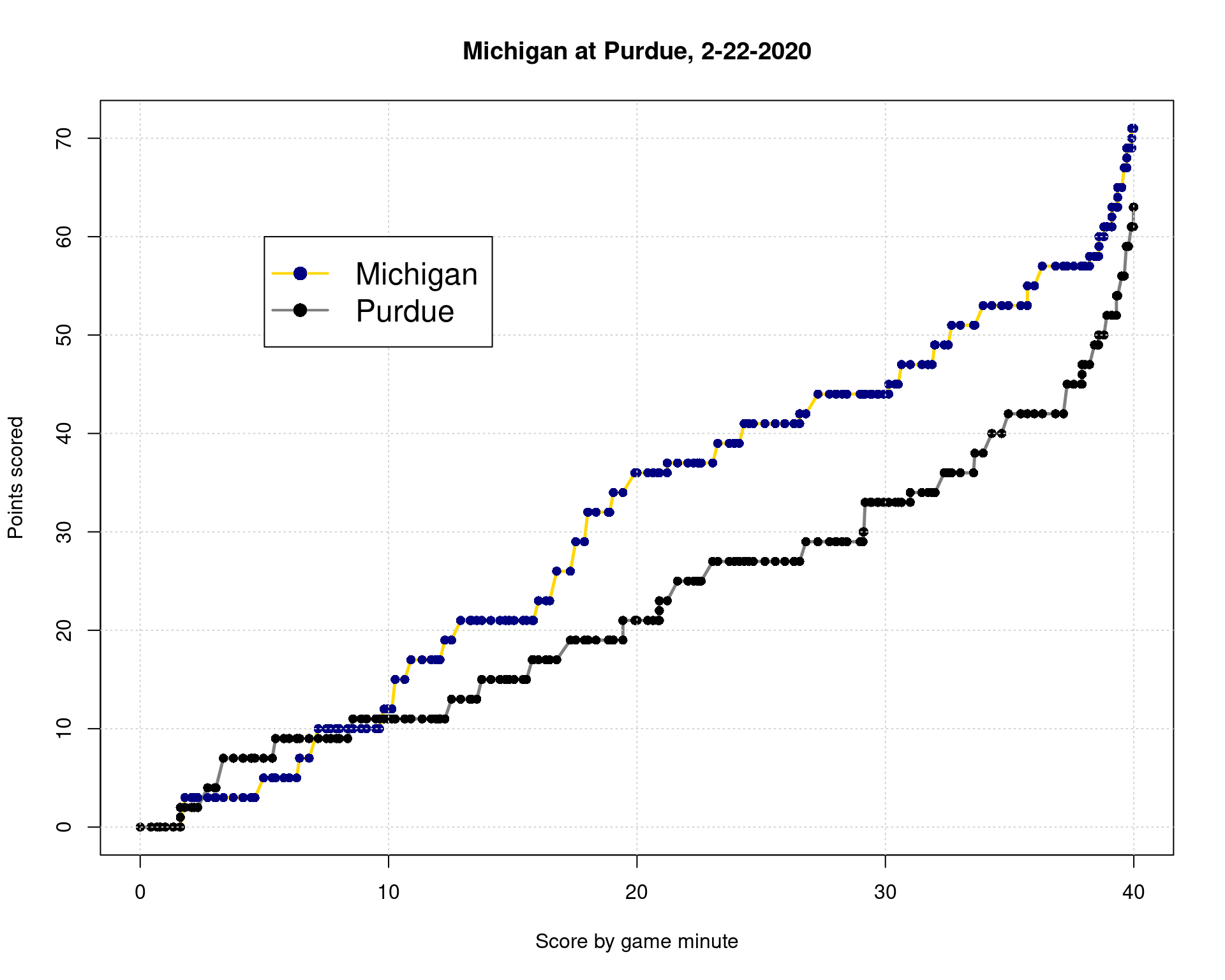
We’d also like to keep track of how many points were scored at each timepoint. Most of the time this will be 0, but sometimes 1, 2, or 3. The original data doesn’t have this in it. I’ll simply calculate the differential and add it to our new data set. This is sort of like how we computed outliers in the body temp data set.
scoredelta <- rbind(c(0,0),
                    scores[-1,] - scores[-nrow(scores),])

matplot(gametime,scoredelta,col=c("navy","black"),type="h")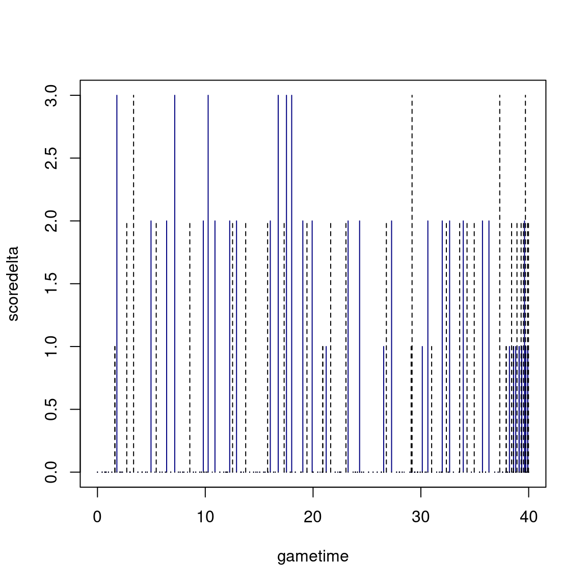
rowSums, colSums, and applyNow that we have some data, let’s say we want to know how many total points were scored, or know the total score (MI+PURDUE) at any time point. Or the average score of both teams at each time point. Previously, we did this with something like scores[,1]+scores[,2], but the rowSums and rowMeans functions do this easily as well, and will work well if we more than two columns
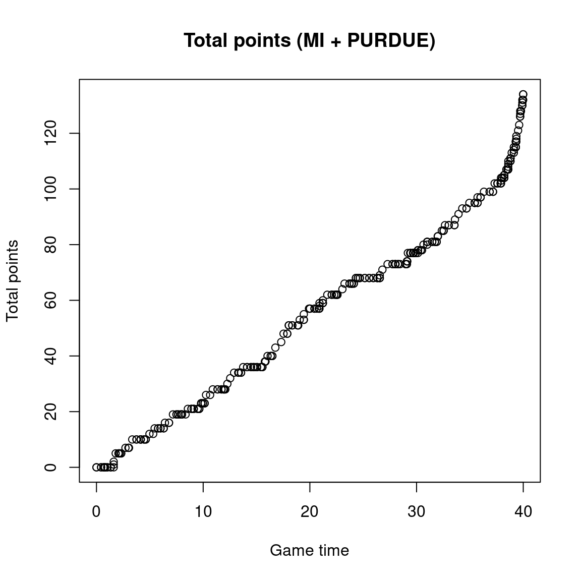
Maybe we want to know the number of points scored during the game by each team. We can use colSums
## MI PU
## 71 63
These are special-purpose functions that apply the function (mean or sum) along all the rows or columns of a matrix or data frame. What if we want to apply a different function, like standard deviation (sd)? We can do the same thing with ```apply’’’, which takes the data frame/matrix, the dimension we want to apply to (1=row, 2=column), and the name of the function
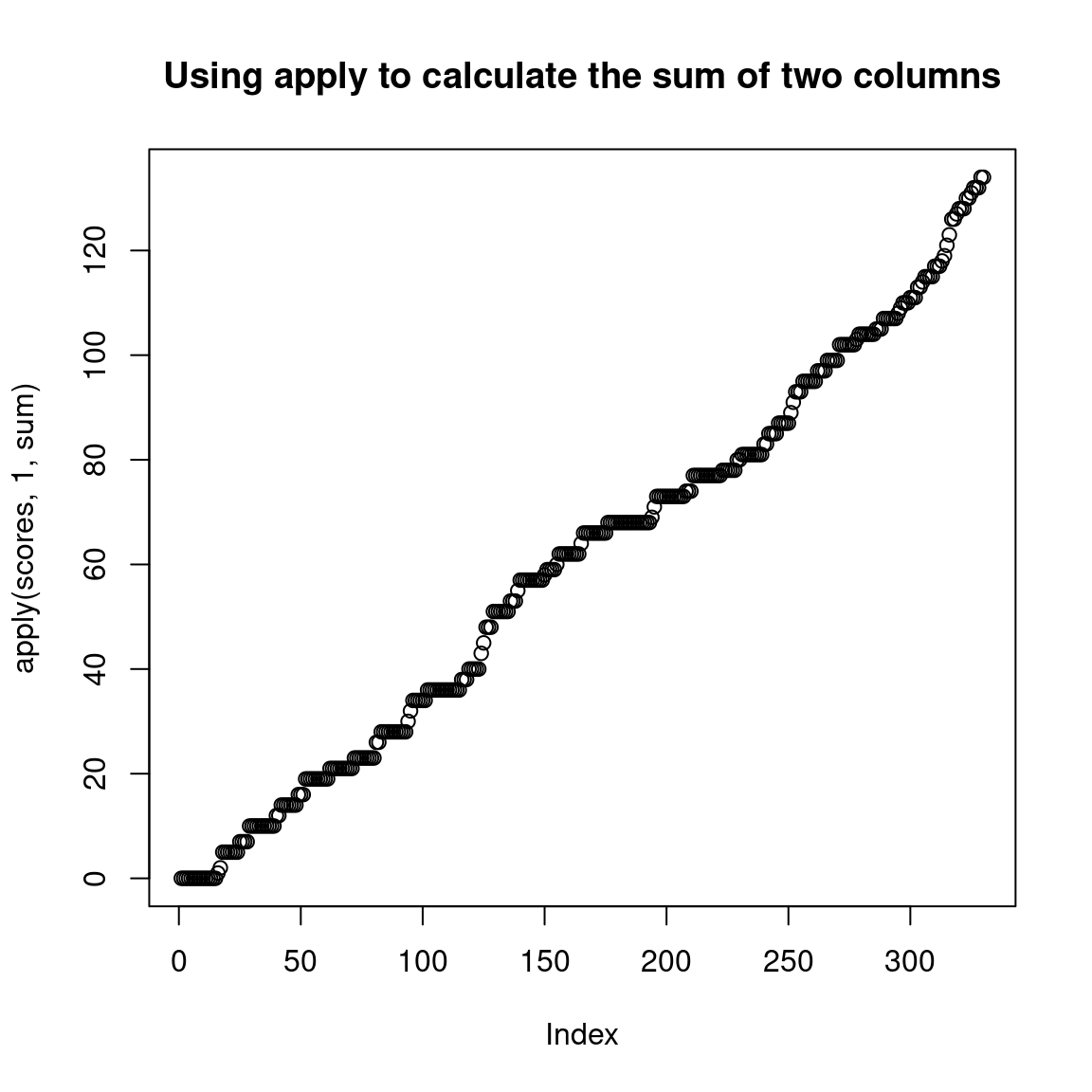
## MI PU
## 71 63## MI PU
## 0.6279320 0.5962719The last one shows the standard deviation of the points earned on each possession change. We’d probably want to filter out to calculate this just for each team’s own possessions, but that
For the following matrix of numbers might be a series of 10 observations made over time of 20 independent participants. We can plot the entire noisy data using matplot. Find the mean, max, and min values of each row, put them together in a data frame and plot them using matplot. Use the add=T argument to overplot these onto the original data.
set.seed(10)
dat <- outer(10+c(1,1.5,1.6,1.9,2.0, 1.2,1.4,1.8,2.1,2.2), 2+runif(20)*1.5) + rnorm(200)*5

matplot(dat,pch=16,cex=.5,col="grey",type="o",lty=1,lwd=.3,
        xlab="Time",ylab="Measured value")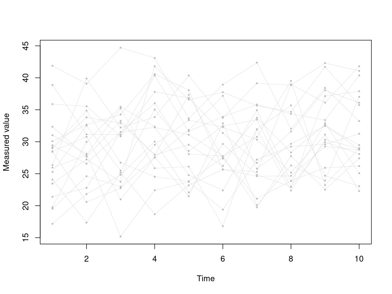
If we have a categorical variables, we often just want to know what the levels are, and how many of them are there. We can use table for that, which will just create an integer vector with the counts of each category, and label each row with the category name. IF we look at the description variable, there might be a lot of unique descriptions of plays, but are there any repetitions? Let’s look. I will use order() to pick out only the most common labels.
## [1] 164##
## Evan Boudreaux Defensive Rebound. Isaiah Livers made Free Throw.
## 12 8
## Official TV Timeout Trevion Williams missed Jumper.
## 7 7
## Trevion Williams Defensive Rebound. Foul on Sasha Stefanovic.
## 6 5
## Franz Wagner Defensive Rebound. Isaiah Livers Defensive Rebound.
## 5 5
## Purdue Defensive Rebound. Zavier Simpson Defensive Rebound.
## 5 5
## Zavier Simpson missed Three Point Jumper. Foul on Austin Davis.
## 5 4
## Foul on Eric Hunter Jr.. Isaiah Livers missed Three Point Jumper.
## 4 4
## Jon Teske missed Jumper. Purdue Timeout
## 4 4
## Sasha Stefanovic Defensive Rebound. Sasha Stefanovic made Free Throw.
## 4 4
## Trevion Williams missed Layup. Trevion Williams Offensive Rebound.
## 4 4It turns out that there were 164 unique descriptions for 330 plays.
In addition, table allows us to calculate cross-tabs: the number of cases that match a pair of IVs. Let’s look at possession_before and shot_outcome variables. It is good to label the row and column to make it easier to interpret:
##           outcome
## team       made missed
##   Michigan   40     48
##   Purdue     34     40
Note that this only adds up to 162, even though there are 300+ plays. The rest of the plays did not end in a shot and were coded as NA; table ignores these NAs by default. But these are interesting in this case, and we can get them back with the useNA argument (check the help).
##           outcome
## team       made missed <NA>
##   Michigan   40     48   77
##   Purdue     34     40   89
##   <NA>        0      0    2
This shows how 89 plays ended for Purdue without a shot, compared to 77 for Michigan. The 2 NA/NA values are probably just the first play of each half, which always end with a possession by one of the teams.
Use table to calculate cross-tabulation of the following variables in bball:
aggregate and tapplyWe often have data organized in columns so that one column is a measure we care about, and other columns are IVs, conditions, or categories we want to organize by. For example, in the basketball data, we can compute a column regarding how many points were scored on any position, which is like a DV. We also have a column showing which team was in possession (bball$shot_team). We often want to collect all the data for each level of an IV, and apply some function to that data set. For example, we might want to find the sum of the points scored by each team. This is what a pivot table in spreadsheet programs permit, but these don’t get used very frequently. There are two common approaches to doing this in R: aggregate and tapply.
We use aggregate when we want to organize functions of one or more DVs by one or more levels of IVs, and we want the resulting table to retain the IV and DV data frame columns. Here are some examples using aggregate and different functions and IVs to compute different statistics about the game:
First, we will calculate the points scored on each possession, and aggregate finding the sum of the points scored by each team. There are two ways to call aggregate, one using a ~formula. The main difference is the name of the values in the data frame.
points <- rowSums(scoredelta)
newdat$points <- points

aggregate(points,list(team=bball$shot_team),sum)
## team x
## 1 Michigan 71
## 2 Purdue 63## shot_team points
## 1 Michigan 71
## 2 Purdue 63This shows the final score was 71 to 63. But what if we also want to know how many points each player scored?
##               player     team  x
## 1       Austin Davis Michigan  3
## 2  Brandon Johns Jr. Michigan  2
## 3     David DeJulius Michigan  6
## 4         Eli Brooks Michigan  4
## 5       Franz Wagner Michigan 22
## 6      Isaiah Livers Michigan 19
## 7          Jon Teske Michigan 11
## 8     Zavier Simpson Michigan  4
## 9      Aaron Wheeler   Purdue  0
## 10   Eric Hunter Jr.   Purdue  7
## 11    Evan Boudreaux   Purdue  4
## 12   Isaiah Thompson   Purdue  5
## 13    Jahaad Proctor   Purdue  6
## 14       Matt Haarms   Purdue  4
## 15     Nojel Eastern   Purdue  6
## 16  Sasha Stefanovic   Purdue 13
## 17  Trevion Williams   Purdue 18
But we might also want to know how many times a player was credited with the possession. We can determine this by finding the length of the vector specified by each combination of team and player:
##               player     team  x
## 1       Austin Davis Michigan  5
## 2  Brandon Johns Jr. Michigan  3
## 3     David DeJulius Michigan  7
## 4         Eli Brooks Michigan  7
## 5       Franz Wagner Michigan 15
## 6      Isaiah Livers Michigan 19
## 7          Jon Teske Michigan 14
## 8     Zavier Simpson Michigan 18
## 9      Aaron Wheeler   Purdue  1
## 10   Eric Hunter Jr.   Purdue 10
## 11    Evan Boudreaux   Purdue  5
## 12   Isaiah Thompson   Purdue  5
## 13    Jahaad Proctor   Purdue  6
## 14       Matt Haarms   Purdue  5
## 15     Nojel Eastern   Purdue  8
## 16  Sasha Stefanovic   Purdue  9
## 17  Trevion Williams   Purdue 25
Similarly, we could calculate average number of points scored per possession by each player by giving it mean instead of length or sum:
##               player     team         x
## 1       Austin Davis Michigan 0.6000000
## 2  Brandon Johns Jr. Michigan 0.6666667
## 3     David DeJulius Michigan 0.8571429
## 4         Eli Brooks Michigan 0.5714286
## 5       Franz Wagner Michigan 1.4666667
## 6      Isaiah Livers Michigan 1.0000000
## 7          Jon Teske Michigan 0.7857143
## 8     Zavier Simpson Michigan 0.2222222
## 9      Aaron Wheeler   Purdue 0.0000000
## 10   Eric Hunter Jr.   Purdue 0.7000000
## 11    Evan Boudreaux   Purdue 0.8000000
## 12   Isaiah Thompson   Purdue 1.0000000
## 13    Jahaad Proctor   Purdue 1.0000000
## 14       Matt Haarms   Purdue 0.8000000
## 15     Nojel Eastern   Purdue 0.7500000
## 16  Sasha Stefanovic   Purdue 1.4444444
## 17 Trevion Williams Purdue 0.7200000tapply to make an aggregate matrixSometimes we want the values aggregated into a table, with levels of one IV along the rows, and another along the columns. This would be nice for making a matplot. The tapply works a lot like aggregate, but organizes the results into a matrix. Here is the same aggregation of points per player.
##                    team
## player              Michigan Purdue
##   Aaron Wheeler           NA      0
##   Austin Davis             3     NA
##   Brandon Johns Jr.        2     NA
##   David DeJulius           6     NA
##   Eli Brooks               4     NA
##   Eric Hunter Jr.         NA      7
##   Evan Boudreaux          NA      4
##   Franz Wagner            22     NA
##   Isaiah Livers           19     NA
##   Isaiah Thompson         NA      5
##   Jahaad Proctor          NA      6
##   Jon Teske               11     NA
##   Matt Haarms             NA      4
##   Nojel Eastern           NA      6
##   Sasha Stefanovic        NA     13
##   Trevion Williams        NA     18
##   Zavier Simpson           4     NA
This would make a lot more sense if the two IVs were not nested like team/player. For example, maybe we want to look at each team or each player and find out how many possessions ended in 0, 1, 2, or 3 points, or how many points were gained in each of those conditions. Using sum as the function will show total point earned by each player/team in each scoring category:
##           gain
## team       0  1  2  3
##   Michigan 0 15 38 18
## Purdue 0 9 42 12## gain
## shooter 0 1 2 3
## Aaron Wheeler 0 NA NA NA
## Austin Davis 0 1 2 NA
## Brandon Johns Jr. 0 NA 2 NA
## David DeJulius 0 1 2 3
## Eli Brooks 0 NA 4 NA
## Eric Hunter Jr. 0 1 6 NA
## Evan Boudreaux 0 2 2 NA
## Franz Wagner 0 1 12 9
## Isaiah Livers 0 8 8 3
## Isaiah Thompson 0 NA 2 3
## Jahaad Proctor 0 NA 6 NA
## Jon Teske 0 NA 8 3
## Matt Haarms 0 NA 4 NA
## Nojel Eastern 0 NA 6 NA
## Sasha Stefanovic 0 4 NA 9
## Trevion Williams 0 2 16 NA
## Zavier Simpson 0 4 NA NAUsing length() will show the number of possessions in each category
##           gain
## team        0  1  2 3
##   Michigan 48 15 19 6
## Purdue 40 9 21 4## gain
## shooter 0 1 2 3
## Aaron Wheeler 1 NA NA NA
## Austin Davis 3 1 1 NA
## Brandon Johns Jr. 2 NA 1 NA
## David DeJulius 4 1 1 1
## Eli Brooks 5 NA 2 NA
## Eric Hunter Jr. 6 1 3 NA
## Evan Boudreaux 2 2 1 NA
## Franz Wagner 5 1 6 3
## Isaiah Livers 6 8 4 1
## Isaiah Thompson 3 NA 1 1
## Jahaad Proctor 3 NA 3 NA
## Jon Teske 9 NA 4 1
## Matt Haarms 3 NA 2 NA
## Nojel Eastern 5 NA 3 NA
## Sasha Stefanovic 2 4 NA 3
## Trevion Williams 15 2 8 NA
## Zavier Simpson 14 4 NA NAWe can see that NAs fill the cells that were empty,
Although college basketball does not have quarters, we can divide the time into 4 equal 10-minute bins we call quarter, which I did above and saved in newdat$quarter. Find the number of points scored by each team in each quarter, using both tapply and aggregate.
##       team quarter  x
## 1 Michigan       1 12
## 2   Purdue       1 11
## 3 Michigan       2 24
## 4   Purdue       2 10
## 5 Michigan       3  8
## 6   Purdue       3 12
## 7 Michigan       4 27
## 8 Purdue 4 30## quarter
## team 1 2 3 4
## Michigan 12 24 8 27
## Purdue 11 10 12 30For a final exercise, let’s try to integrate several of these.
##   [1]   1   2   3   4   5   6   7   8   9  10  11  12  13  14  15  16  17  18  19  20  21  22  23  24  25  26  27  28  29
##  [30]  30  31  32  33  34  35  36  37  38  39  40  41  42  43  44  45  46  47  48  49  50  51  52  53  54  55  56  57  58
##  [59]  59  60  61  62  63  64  65  66  67  68  69  70  71  72  73  74  75  76  77  78  79  80  81  82  83  84  85  86  87
##  [88]  88  89  90  91  92  93  94  95  96  97  98  99 100 101 102 103 104 105 106 107 108 109 110 111 112 113 114 115 116
## [117] 117 118 119 120 121 122 123 124 125 126 127 128 129 130 131 132 133 134 135 136 137 138 139 140 141 142 143 144 145
## [146] 146 147 148 149 150 151 152 153 154 155 156 157 158 159 160 161 162 163 164 165 166 167 168 169 170 171 172 173 174
## [175] 175 176 177 178 179 180 181 182 183 184 185 186 187 188 189 190 191 192 193 194 195 196 197 198 199 200 201 202 203
## [204] 204 205 206 207 208 209 210 211 212 213 214 215 216 217 218 219 220 221 222 223 224 225 226 227 228 229 230 231 232
## [233] 233 234 235 236 237 238 239 240 241 242 243 244 245 246 247 248 249 250 251 252 253 254 255 256 257 258 259 260 261
## [262] 262 263 264 265 266 267 268 269 270 271 272 273 274 275 276 277 278 279 280 281 282 283 284 285 286 287 288 289 290
## [291] 291 292 293 294 295 296 297 300 301 302 303 304 305 306 307 308 309 310 311 312 313 314 315 316 317 318 319 320 321
## [320] 322 323 324 325 326 327 328 329 330 331 332## Aaron Wheeler Austin Davis Brandon Johns Jr. David DeJulius Eli Brooks Eric Hunter Jr. Evan Boudreaux Franz Wagner
## 20 0 0 0 0 0 0 0 0
## 21 0 0 0 0 0 0 0 0
## 22 0 0 0 0 0 0 0 0
## 23 0 0 0 0 0 0 0 0
## 24 0 0 0 0 0 0 0 0
## 25 0 0 0 0 0 0 0 0
## 26 0 0 0 0 0 0 0 0
## 27 0 0 0 0 0 0 0 0
## 28 0 0 0 0 0 0 0 0
## 29 0 0 0 0 0 0 0 0
## 30 0 0 0 0 0 0 0 0
## Isaiah Livers Isaiah Thompson Jahaad Proctor Jon Teske Matt Haarms Nojel Eastern Sasha Stefanovic Trevion Williams
## 20 0 0 0 0 0 0 0 0
## 21 0 0 0 0 0 0 0 0
## 22 0 0 0 0 0 0 0 0
## 23 0 0 0 0 0 0 0 0
## 24 0 0 0 0 0 0 0 0
## 25 0 0 2 0 0 0 0 0
## 26 0 0 0 0 0 0 0 0
## 27 0 0 0 0 0 0 0 0
## 28 0 0 0 0 0 0 0 0
## 29 0 0 0 0 0 0 3 0
## 30 0 0 0 0 0 0 0 0
## Zavier Simpson
## 20 0
## 21 0
## 22 0
## 23 0
## 24 0
## 25 0
## 26 0
## 27 0
## 28 0
## 29 0
## 30 0##
## Michigan Purdue
## Aaron Wheeler 0 1
## Austin Davis 5 0
## Brandon Johns Jr. 3 0
## David DeJulius 7 0
## Eli Brooks 7 0
## Eric Hunter Jr. 0 10
## Evan Boudreaux 0 5
## Franz Wagner 15 0
## Isaiah Livers 19 0
## Isaiah Thompson 0 5
## Jahaad Proctor 0 6
## Jon Teske 14 0
## Matt Haarms 0 5
## Nojel Eastern 0 8
## Sasha Stefanovic 0 9
## Trevion Williams 0 25
## Zavier Simpson 18 0Let’s create a vector which tells us which team each player plays for.
##     Aaron Wheeler      Austin Davis Brandon Johns Jr.    David DeJulius        Eli Brooks   Eric Hunter Jr.
##                 2                 1                 1                 1                 1                 2
##    Evan Boudreaux      Franz Wagner     Isaiah Livers   Isaiah Thompson    Jahaad Proctor         Jon Teske
##                 2                 1                 1                 2                 2                 1
##       Matt Haarms     Nojel Eastern  Sasha Stefanovic  Trevion Williams    Zavier Simpson
##                 2                 2                 2                 2                 1
Next, we can use apply with cumsum to look at cumulative points for each player. This looks like magic, but what we are doing is finding the cumulative sum of values in each column, for each column separately. We can use team.membership to color each series, and put player names based on their final points at the right side.
cumulative.pbp <- apply(playerbyplay,2,cumsum)

purdue.cumulative <- cumsum(rowSums(playerbyplay[,team.membership==2]))
michigan.cumulative <- cumsum(rowSums(playerbyplay[,team.membership==1]))

matplot(gametime,cumulative.pbp,type="l",col=c("blue","black")[team.membership],lty=1,main="Cumulative points scored by each player",
        xlab="Game time",ylab="Cumulative points",xlim=c(0,50),ylim=c(0,70))
lines(gametime,purdue.cumulative,lwd=3,col="black")
lines(gametime,michigan.cumulative,lwd=3,col="blue")

grid()
legend(0,60,c("Michigan player","Purdue player"),col=c('blue','black'),lty=1)

finalpoints <- aggregate(points,list(player=bball$shooter),sum)

text(41,finalpoints$x,finalpoints$player,pos=4,cex=.7,col=c("blue","black")[team.membership])
text(41,max(michigan.cumulative),"Michigan",pos=4)
text(41,max(purdue.cumulative),"Purdue",pos=4)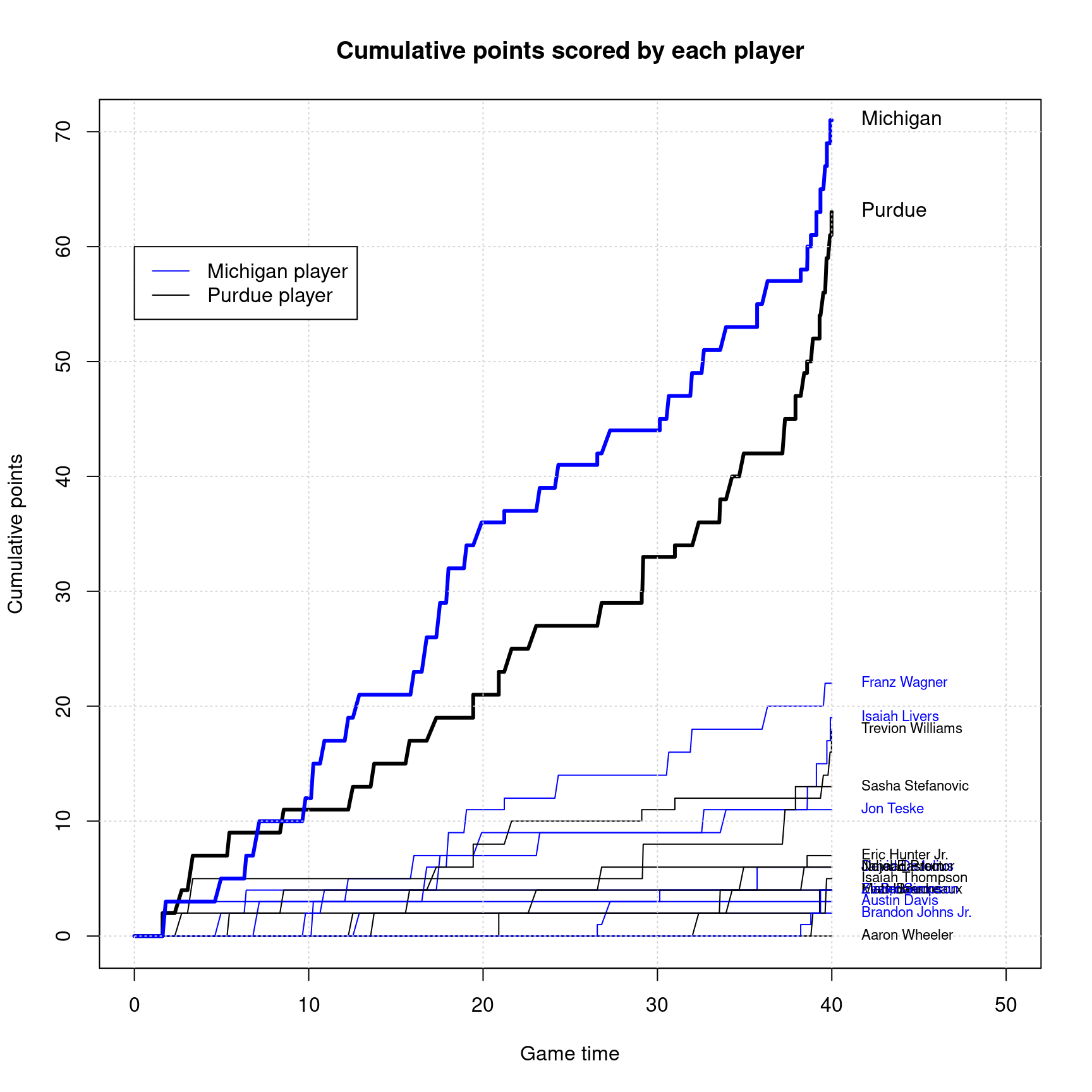
This isn’t perfect because we have player names overlapping, but it shows how we used apply, tapply, aggregate, and rowSums, all together to create a comprehensive look at the game.
Use table to calculate cross-tabulation of:
For each one, try to explain what the table is telling you.
##           after
## before     Michigan Purdue
##   Michigan       59    105
## Purdue 113 49## freethrow
## team FALSE TRUE
## Michigan 65 23
## Purdue 62 12## three
## team FALSE TRUE
## Michigan 63 25
## Purdue 59 15## outcome
## player made missed
## Aaron Wheeler 0 1
## Austin Davis 2 3
## Brandon Johns Jr. 1 2
## David DeJulius 3 4
## Eli Brooks 2 5
## Eric Hunter Jr. 4 6
## Evan Boudreaux 3 2
## Franz Wagner 10 5
## Isaiah Livers 13 6
## Isaiah Thompson 2 3
## Jahaad Proctor 3 3
## Jon Teske 5 9
## Matt Haarms 2 3
## Nojel Eastern 3 5
## Sasha Stefanovic 7 2
## Trevion Williams 10 15
## Zavier Simpson 4 14For the following matrix of numbers might be a series of 10 observations made over time of 20 independent participants. We can plot the entire noisy data using matplot. Find the mean, max, and min values of each row, put them together in a data frame and plot them using matplot. Use the add=T argument to overplot these onto the original data.
set.seed(10)
dat <- outer(10+c(1,1.5,1.6,1.9,2.0, 1.2,1.4,1.8,2.1,2.2), 2+runif(20)*1.5) + rnorm(200)*5

matplot(dat,pch=16,cex=.5,col="grey",type="o",lty=1,lwd=.3,
        xlab="Time",ylab="Measured value")


summarydat <- data.frame(mean=rowMeans(dat),
                         min=apply(dat,1,min),
                         max=apply(dat,1,max))


matplot(summarydat,add=T,type="l",lwd=3,lty=c(1,3,3))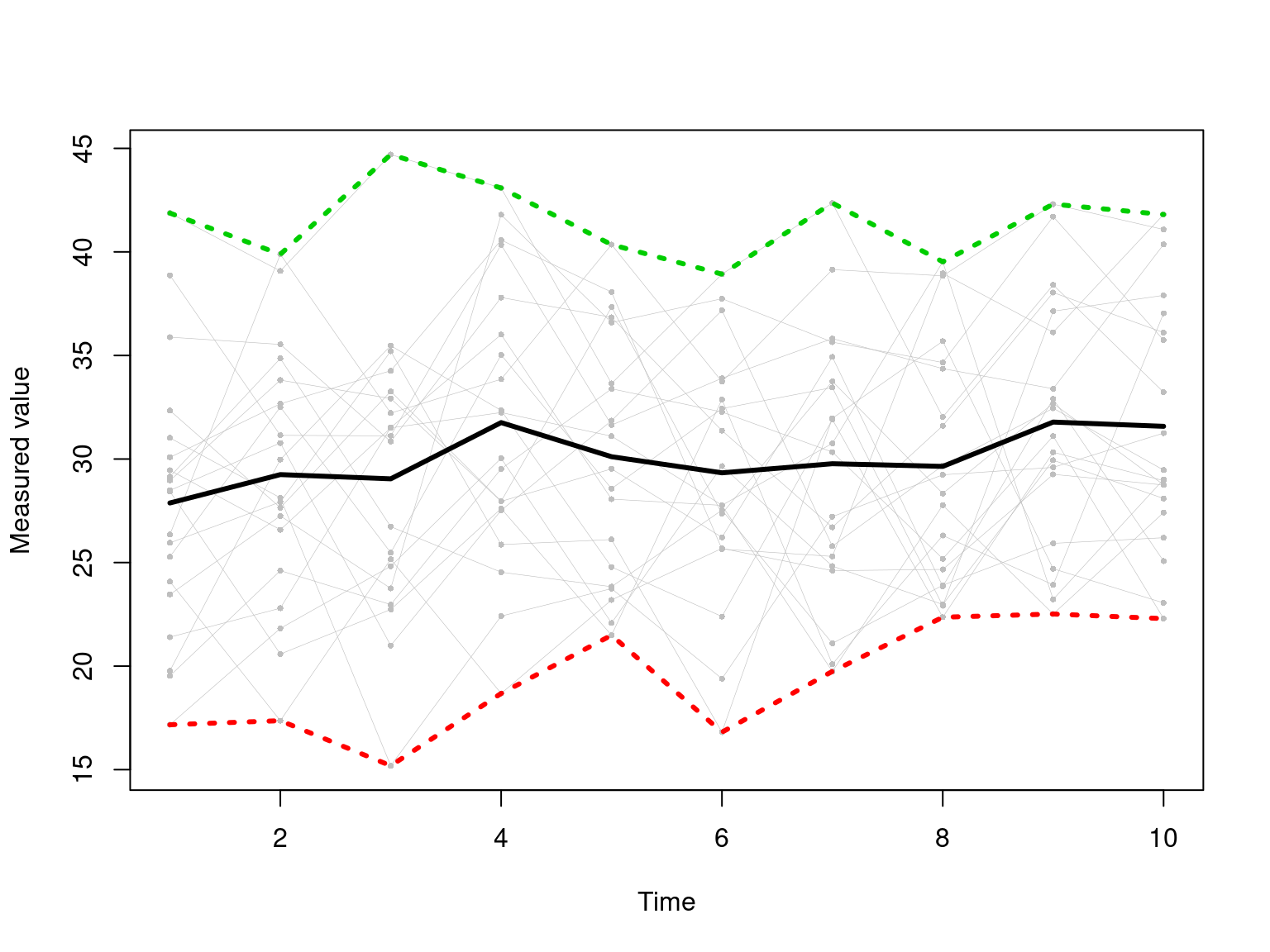
Although college basketball does not have quarters, we can divide the time into 4 equal 10-minute bins we call quarter, which I did above and saved in newdat$quarter. Find the number of points scored by each team in each quarter, using both tapply and aggregate.
##           quarter
## team        1  2  3  4
##   Michigan 18 17 21 32
## Purdue 18 16 15 25## quarter team x
## 1 1 Michigan 18
## 2 2 Michigan 17
## 3 3 Michigan 21
## 4 4 Michigan 32
## 5 1 Purdue 18
## 6 2 Purdue 16
## 7 3 Purdue 15
## 8 4 Purdue 25